
Process Scheduling (via wikipedia) is defined as:
The method by which threads, processes or data flows are given access to system resources (e.g. processor time, communications bandwidth). This is usually done to load balance and share system resources effectively or achieve a target quality of service. The need for a scheduling algorithm arises from the requirement for most modern systems to perform multitasking (executing more than one process at a time) and multiplexing (transmit multiple data streams simultaneously across a single physical channel).
In other words, process scheduling refers to algorithms which allocate resources (this includes CPU, Memory, Disk, etc.) to processes/threads at a given time. Throughout this article I am going to refer to processes attempting to obtain resources, but it could be threads as well.
Purpose
The goal of the article is to give an introduction to process scheduling. The idea being that a basic understanding of definitions and the most basic algorithms will help you grasp the more complex scheduling algorithms.
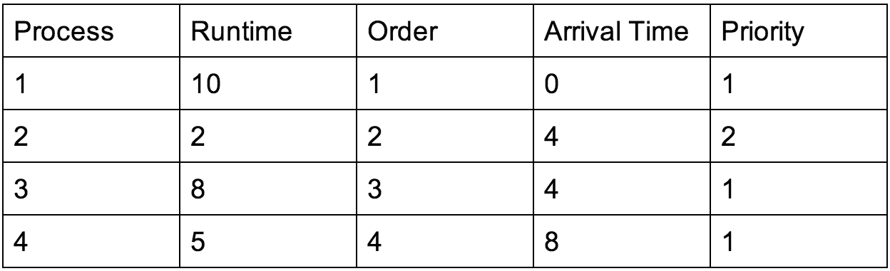
The various examples will use the following table of processes, arrival times (the time at which the process requested access), and runtimes:
Definitions
- Response Time: How long it takes for the process to run for the first time.
- Wait Time: The total amount of time a process does not have access to the resource(s), since the first access.
- Average Wait Time: The average time spent between regaining access to the resource(s).
- Starvation: When a process never gains access to a given resource.
Batch Scheduling Algorithms
Batch scheduling refers to non-preemptive algorithms, meaning there are no interruptions to a process once it gains access to a resource until that process is finished.
FCFS
FCFS – First Come First Server
In this algorithm the first process to request access to a resource receive access to the resource, this refers to the “order” of requests. Using the table above, the times each process gained access to a resource are as follows:
Time Intervals:
Process 1: 0 – 10
Process 2: 10 – 12
Process 3: 12 – 20
Process 4: 20 – 25
Total Runtime: 25
If we then wish to analyze how well the algorithm has worked, we would look at the wait times and/or priority. In this case, lets assume that each process has equal priority.
Time Waiting:
Process 1: 0
Process 2: 6 (arrived at 4, waited until 10)
Process 3: 8 (arrived at 4, waited until 12)
Process 4: 12 (arrived at 8, waited until 20)
Total Time Waiting: 26
Average Time Waiting:
26 / 4 = 6.5
As you can see this algorithm does nothing to reduce waiting time. Worse, a single long process can maintain access to the resource for a prolonged period and multiple short jobs must wait.
There are specific cases where, for example, one process needs access to the CPU and one needs access to disk, but if there is an exceptionally long process that needs access to the disk, the process that needs access to the CPU rarely obtains it. This leads to another algorithm, called…
SJF/SJN
SJF/SJN – Shortest Job First/Next
In this algorithm the job with the shortest remaining time runs, this algorithm is based off “time” as opposed to order of the requests:
Time Intervals:
Process 1: 0 – 10
Process 2: 10 – 12
Process 3: 17 – 25
Process 4: 12 – 17
Total Runtime: 25
Lets again look at the wait time(s) to analyze how effective this algorithm is:
Time Waiting:
Process 1: 0
Process 2: 6 (arrived at 4, waited until 10)
Process 3: 9 (arrived at 4, waited until 17)
Process 4: 4 (arrived at 8, waited until 12)
Total Time Waiting: 19
Average Waiting Time:
19 / 4 = 4.75
Compared to the FCFS algorithm we have significantly reduced the total time waiting, however there is a major problem with this algorithm. With SJF it is possible to continuously receive processes with a short run time that can effectively starve the other processes (i.e. they never gain access to the resources). This is very bad if response time important.
Pre-Emptive Scheduling Algorithms
Preemptive scheduling refers to temporarily interrupting a given process via a signal (of some kind) to run a different process, later returning to the original process.
Round-Robin
For Round-Robin we split time into quanta (or time increments), each process is then given a quanta on which it runs. For example, if there are just two processes, process one may run on odd milliseconds and process two runs on even milliseconds. This may mean a given process takes longer to finish, but it ensures that every process gains some access to the resource and it eliminates excessive wait times and the possibility of starvation.
If we ran it on the above table of processes with a quanta of 2 time interval:
Time Intervals:
Process 1: 0 – 4 (It is the only process until 4, 6 remaining)
Process 2: 4 – 6 (0 remaining)
Process 3: 6 – 8 (6 remaining)
Process 4: 8 – 10 (3 remaining)
Process 1: 10 – 12 (4 remaining)
Process 3: 12 – 14 (4 remaining)
Process 4: 14 – 16 (1 remaining)
Process 1: 16 – 18 (2 remaining)
Process 3: 18 – 20 (2 remaining)
Process 4: 20 – 21 (0 remaining)
Process 1: 21 – 23 (0 remaining)
Process 3: 23 – 25 (0 remaining)
Total Runtime: 25
For Round-Robin there is always some wait times if there are multiple processes, with at least one having a run time greater than the quanta.
Time Waiting:
Process 1: 13
Process 2: 8
Process 3: 11
Process 4: 8
Total Time Waiting: 40
Average Wait Time:
Process 1: 13 / 4 = 4.3333..
Process 2: 0
Process 3: 11 / 4 = 2.75
Process 4: 8 / 3 = 2.66666
Total: (4.333 + 0 + 2.75 + 2.66666) / 4 = 2.437
This is by far the longest total time spent waiting, and unfortunately is quite common with the Round-Robin method of scheduling, but it also has the lowest average waiting time by a significant margin. This is why round-robin works well for processes which run constantly, but not for processes for which the final execution is most important. For example, Round-Robin would work fine for updating a GUI (graphical user interface) because it is something that consistently needs to happen. On the other hand a complex calculation where only the final result matters would take much longer while using the Round-Robin algorithm of scheduling (if other processes are also running).
One of the tricks for Round-Robin is picking a correct time quantum, if you pick to short a time quantum it becomes inefficient due to the overhead of switching out processes. On the other hand, if you pick to long of a time quantum it essentially becomes a FCFS. A good “rule of thumb” is 70 – 80 % of block within the time quantum.
Priority Pre-Emptive Scheduling
As the name suggests, this algorithm allocates resources based on the priority of the given process. If two processes have the same priority most systems switch to Round-Robin and force the processes to take turns.
If we were to run this algorithm on the table above we would get:
Time Intervals:
Process 1: 0 – 4 (priority 1 – 6 remaining)
Process 3: 4 – 6 (priority 1 – 6 remaining)
Process 1: 6 – 8 (priority 1 – 4 remaining)
Process 4: 8 – 10 (priority 1 – 3 remaining)
Process 3: 10 – 12 (priority 1 – 4 remaining)
Process 1: 12 – 14 (priority 1 – 2 remaining)
Process 4: 14 – 16 (priority 1 – 1 remaining)
Process 3: 16 – 18 (priority 1 – 2 remaining)
Process 1: 18 – 20 (priority 1 – 0 remaining)
Process 4: 20 – 21 (priority 1 – 0 remaining)
Process 3: 21 – 23 (Priority 1 – 0 remaining)
Process 2: 23 – 25 (Priority 2 – 0 remaining)
Total Runtime: 25
Because priority pre-emptive scheduling is minimizing the top priorities wait time as opposed to average wait time, it is difficult to determine whether this is “better” or not when comparing.
Time Waiting:
Process 1: 10
Process 2: 23
Process 3: 11
Process 4: 8
Total Time Waiting: 52
Average Wait Time:
Process 1: 10 / 4 = 2.5
Process 2: 23
Process 3: 11 / 4 = 2.75
Process 4: 8 / 3 = 2.6666..
Total: (2.5 + 23 + 2.75 + 2.66666) / 4 = 7.729
When comparing the average time spent waiting, it is clear that this is by far the worst scheduling algorithm. However, if we look purely at how long the priority ones have to wait:
Priority 1: Average Wait Time:
(2.5 + 2.75 + 2.6666) / 3 = 2.639
This would make the average wait time for the highest priority lower than any of the above algorithms. This could be useful in some applications, such as emergency systems where an application can run in Round-Robin, but if something goes wrong a higher priority process comes in and takes over. An example of this system could be an auto-brake on a self-driving car, or an automatic shutdown on a rocket about to take off.
It would not be in your best interest to use this algorithm however, if priority is not your primary concern. Take the example above, if (as a programmer) you are trying to optimize for fairness in the sense that you minimize overall waiting time or average waiting time. It would not make sense to use priority pre-emptive scheduling because starvation can occur in this system if you receive many/constant high priority processes and occasionally a low priority process (the low priority processes will never be ran).
Related Articles