
Everyday Algorithms:
This may be a bit of a divergence from my regular “Everyday Algorithms” series, however I feel it is important. Thus far, most algorithm’s I have discussed have been directly related to real life events. I.e. flipping pancakes, planning a road trip, etc. That being said, I feel it is important to cover binary trees. They have many real world applications and are fundamental to many of the future algorithms I have in mind.
What is a Binary Tree?
Binary trees may have real world applications, but are slightly abstract. A binary tree is what we call a data structure, and as the name implies, it structures input data in a way that makes it easier to extract meaning.
This means, that it should be easier to find whether or not a particular number is apart of a given set in a data structure than it would be without structure. An example of a binary search tree, which is a binary tree with the property that it can easily be searched, (described in detail later), would look something like this:
Input: { 40, 4, 34, 45, 14, 55, 48, 13, 15, 49, 47 }
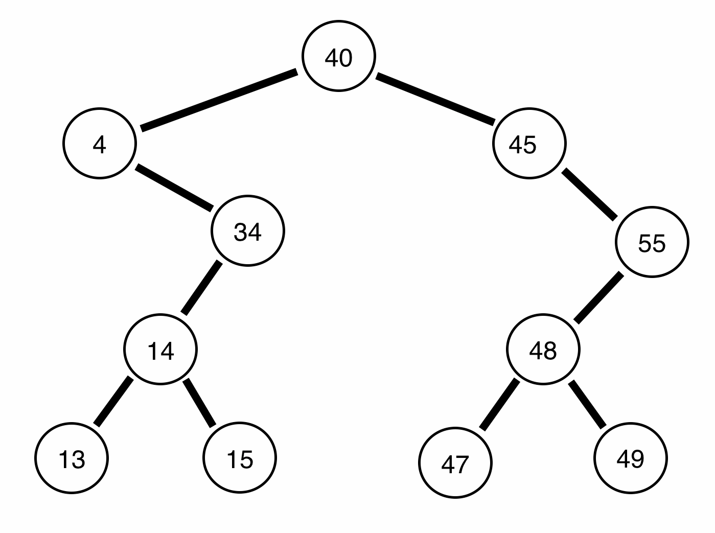
Abstractly, a binary tree consists of a node, called a root. In the above image, the root would be 40. We then attach to that root node other nodes as they come in. So, for example if we take the input above, { 40, 4, 34, 45, 14, 55, 48, 13, 15, 49, 47 }, the first node is the root node, which is 40. After we place that in the root, we then look to place the value 4.
Now, there are various ways to set up binary trees, all with various benefits. For example,
We could always place nodes larger than the root to the right, and nodes smaller than the root to the left.
This article will only contain examples referencing rooted binary search trees, using the above rule, however, it is good to know other methods of binary tree construction are available (i.e. balanced, infinite, perfect, etc.)[1].
Constructing a Binary Tree
If we follow these rules,
- We always place nodes larger than the root to the right, and nodes smaller than the root to the left
- If no spaces are available set root to be the node closest to the new input value
- Repeat
With the following input,
Input: { 40, 4, 34, 45, 14, 55, 48, 13, 15, 49, 47 }
We can construct the tree as follows:
Say, we wished to program this, it would be relatively straight forward in python. First, by creating a node class which can handles to left or right node objects, then another variable to store the data. Second, we can create a binary tree class, which simply contains a root and functions to construct the tree (code on my github):
Why Use a Data Structure?
So, why should we use data structures? It seems like a lot of extra work, and what are the benefits?
Let us assume we have an arbitrary set of numbers, call this set S, and we wanted to determine whether or not it contained a particular value, we would have to check every single number. This means the “runtime” of our algorithm will be the size of S (all of the numbers in the set). If we were to use big-O notation, which is often used to represent runtime, it would be O(n), where n is the number of numbers in set S.
Alternatively, if we apply some structure to the set of numbers S, we may be able to find the numbers faster. Say, for example, if we sort the numbers from smallest to largest. If we are searching for number x in the set of numbers, we can start from the beginning, and go until we reach the number we are looking for, OR the number greater than it. Thereby giving us a runtime, on average, less than the runtime of checking every number in the set S.
If we use construct binary search tree, we can even get better time. Take a moment to consider why…
Searching a Binary Tree
Notice, that because we know every number to the left of the root node is smaller than the root node, and every node to the right of the root node is larger. We can quickly search through and discover whether or not a particular number is apart of a set in very few steps (much quicker than even a sorted list).
The average runtime of search in a binary search tree is on average O(log(n)). In other words, it requires us to check only half of the nodes at each level (i.e. do we go left or right). However, in the worse case, you could have a set of numbers such as { 40, 45, 55 } in which case, all of the numbers would be in a straight list (view the image above for reference) in this case the runtime would be O(n).
If we wished to program this, it would be relatively straight forward. Essentially, we would check to see if
- Does the current node contain the value we are looking for?
- If we are not, is the value were are looking less than the root or more than the root
- Then move to the appropriate side
- Repeat until node is discovered, or we reach the end
In python would look like (github):
Deletion in a Binary Tree
I will not be providing code for this section, as I feel it is an excellent exercise for the reader. Think about how you would delete a node, but be careful… There are a few tips on wikipedia.
Pre-Order Traversal of a Binary Tree
What is a traversal? In the case of binary trees, it is the act of visiting each node and outputting or storing the data in the node. For example, if we always go as far as we can left, then as far as we can right, this is called a pre-order traversal.
If we were to visually represent this with our sample set:

Notice, we are always attempting to go as far as we can left before we go right, and always printing the node we are on prior to continuing. This is the entire concept of pre-order traversals, think of it as going as far as we can PREVIOUS to the root, then going POST to the root value. If we were to see this in code form (on github):
Post-Order Traversal of a Binary Tree
Post-order traversals are extremely similar to pre-order traversals. The only difference being when you print or store the data. Instead of printing prior to exploring each of the possible trees, the algorithm prints after all nodes have been explored, effectively printing out the tree in reverse. Take for example our input,
Input: { 40, 4, 34, 45, 14, 55, 48, 13, 15, 49, 47 }
The output of this tree in post-order traversal will be as follows,
Output: { 13, 15, 14, 34, 4, 47, 49, 48, 55, 45, 40 }
Was it what you were expecting? Here’s a visualization to help you:

The purple represents when the numbers should print out, the red represents the current root, and the orange represents the prior root of the function which called the current root. I know that can be a bit confusing, but after you review the code it may become more clear (on github):
As you can see, the print function is not called until all left and right nodes are traversed, which is why our root node (40) is the last to be printed. I would also like to point out that the runtime of this algorithm is still O(n), since we only visit each node once.
Ordered Traversal of a Binary Tree
Ordered traversal are as the name sounds, in order. The only adjustment to the algorithm is that we print/store each nodes value after we visit all the nodes to the left of it. Review below to witness a visualization:
Note, we will output the tree in sorted order perfectly: { 4, 13, 14, 15, 34, 40, 45, 47, 48, 49, 55 }! If you want to see the code, it is very similar to before, only that we are printing between left and right calls (on github):
Level Order Traversal of a Binary Tree
This one is a bit more tricky. Imagine that we wanted to print out every level of the binary tree, that is to say given,
Input: { 40, 4, 34, 45, 14, 55, 48, 13, 15, 49, 47 }
We would like to output something like,
{ 40 }
{ 4, 45 }
{ 34, 55 }
{ 14, 48 }
{ 13, 15, 47, 49 }
We cannot use our same method, as we did before. Instead, we will use something called a queue, and a method called Bredth-First search. Rather than diving into what each of those are, I will leave you to read about them yourself, and provide a nice visual below:
As you can see it’s pretty effective, although moderately hard to understand without knowledge of Beadth-first Search. Essentially, we store each previous level in a abstract data type called a queue. In a queue, you can “pop” off the front and receive the first node you stored inside of it (which is why a queue is called a FIFO – First In First Out). Once we pop a node, we add its children (left and right nodes) to the queue and print the node. You can review this in python below (on github):
Please note that the runtime of this algorithm is still O(n), in big-O notation, since we only ever visit a node once. After we pop the node from the queue.
Closing Commentary
There are loads of uses for binary trees, ancestry charts, decision trees, potentially psychiatry, etc. It is one of the most fundamental data structures, and it is essential for any blossoming programmer to fully understand how they work. Further, these are not the only traversals, or even types of binary trees, and I highly recommend reading more about various types if you are interested!
If you enjoyed this article I recommend signing up for my mailing list, or reading one of my related articles below!
Hi Austin,
Can you please let me know what is the name of the algorithm which uses all the operations (tree traversals) in a binary tree?
Regards,
Srini.